Timing Graph Debugging Tutorial
When developing VPR or creating/calibrating the timing characteristics of a new architectural model it can be helpful to look ‘inside’ at VPR’s timing graph and analysis results.
Warning
This is a very low-level tutorial suitable for power-users and VTR developers
Generating a GraphViz DOT file of the Entire Timing Graph
One approach is to have VPR generate a GraphViz DOT file, which visualizes the structure of the timing graph, and the analysis results.
This is enabled by running VPR with vpr --echo_file set to on.
This will generate a set of .dot files in the current directory representing the timing graph, delays, and results of Static Timing Analysis (STA).
$ vpr $VTR_ROOT/vtr_flow/arch/timing/EArch.xml $VTR_ROOT/vtr_flow/benchmarks/blif/multiclock/multiclock.blif --echo_file on

$ ls *.dot
timing_graph.place_final.echo.dot  timing_graph.place_initial.echo.dot  timing_graph.pre_pack.echo.dot
The .dot files can then be visualized using a tool like xdot which draws an interactive version of the timing graph.
$ xdot timing_graph.place_final.echo.dot
Warning
On all but the smallest designs the full timing graph .dot file is too large to visualize with xdot. See the next section for how to show only a subset of the timing graph.
Which will bring up an interactive visualization of the graph:
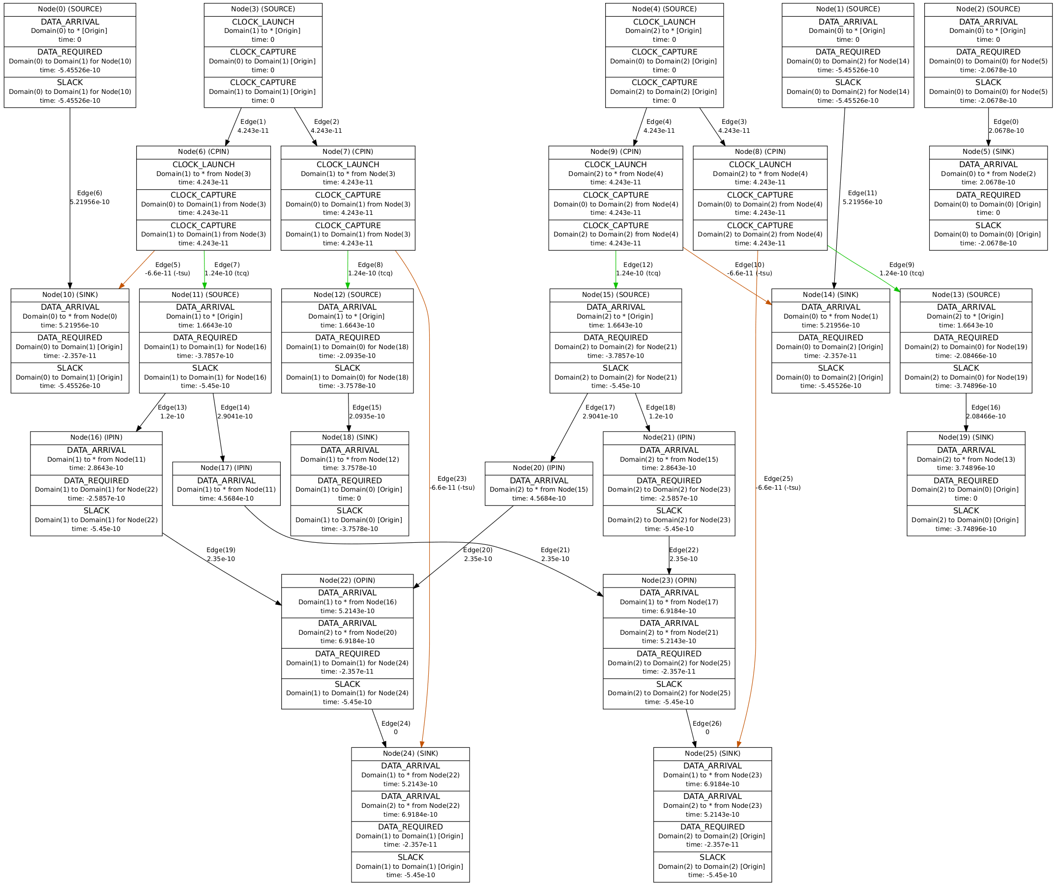
Fig. 97 Full timing graph visualized with xdot on a very small multi-clock circuit.
Where each node in the timing graph is labeled
Node(X) (TYPE)
Where Node(X) (e.g. Node(3)) represents the ID of the timing graph node, and (TYPE) (e.g. OPIN) is the type of node in the graph.
Each node is also annotated with timing information (produced by STA) like
DATA_ARRIVAL
Domain(1) to * from Node(16)
time: 5.2143e-10

DATA_ARRIVAL
Domain(2) to * from Node(20)
time: 6.9184e-10

DATA_REQUIRED
Domain(1) to Domain(1) for Node(24)
time: -2.357e-10

SLACK
Domain(1) to Domain(1) for Node(24)
time: -5.45e-10
where the first line of each entry is the type of timing information (e.g. data arrival time, data required time, slack),
the second line indicates the related launching and capture clocks (with * acting as a wildcard) and the relevant timing graph node which originated the value,
and the third line is the actual time value (in seconds).
The edges in the timing graph are also annotated with their Edge IDs and delays.
Special edges related to setup/hold (tsu, thld) and clock-to-q delays (tcq) of sequential elements (e.g. Flip-Flops) are also labeled and drawn with different colors.
Generating a GraphViz DOT file of a subset of the Timing Graph
For most non-trivial designs the entire timing graph is too large and difficult to visualize.
To assist this you can generate a DOT file for a subset of the timing graph with vpr --echo_dot_timing_graph_node
$ vpr $VTR_ROOT/vtr_flow/arch/timing/EArch.xml $VTR_ROOT/vtr_flow/benchmarks/blif/multiclock/multiclock.blif --echo_file on --echo_dot_timing_graph_node 23
Running xdot timing_graph.place_final.echo.dot now shows the only the subset of the timing graph which fans-in or fans-out of the specified node (in this case node 23).
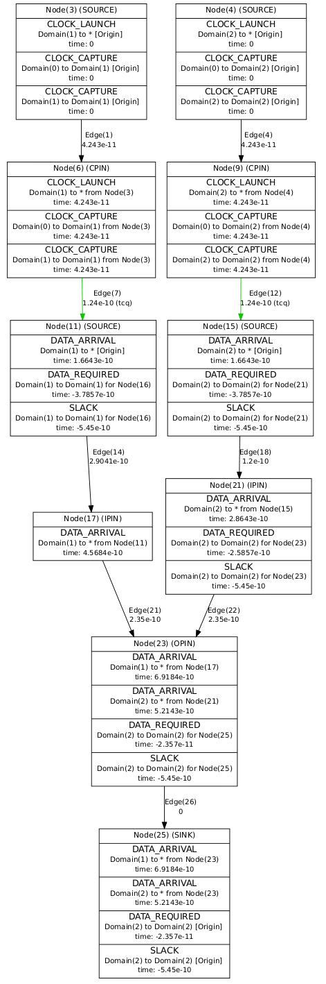
Fig. 98 Subset of the timing graph which fans in and out of node 23.
Cross-referencing Node IDs with VPR Timing Reports
The DOT files only label timing graph nodes with their node IDs. When debugging it is often helpful to correlate these with what are seen in timing reports.
To do this, we need to have VPR generate more detailed timing reports which have additional debug information.
This can be done with vpr --timing_report_detail set to debug:
$ vpr $VTR_ROOT/vtr_flow/arch/timing/EArch.xml $VTR_ROOT/vtr_flow/benchmarks/blif/multiclock/multiclock.blif --timing_report_detail debug

$ ls report_timing*
report_timing.hold.rpt report_timing.setup.rpt
Viewing report_timing.setup.rpt:
#Path 6
Startpoint: FFB.Q[0] (.latch at (1,1) tnode(15) clocked by clk2)
Endpoint  : FFD.D[0] (.latch at (1,1) tnode(25) clocked by clk2)
Path Type : setup

Point                                                             Incr      Path
--------------------------------------------------------------------------------
clock clk2 (rise edge)                                           0.000     0.000
clock source latency                                             0.000     0.000
clk2.inpad[0] (.input at (3,2) tnode(4))                         0.000     0.000
| (intra 'io' routing)                                           0.042     0.042
| (inter-block routing:global net)                               0.000     0.042
| (intra 'clb' routing)                                          0.000     0.042
FFB.clk[0] (.latch at (1,1) tnode(9))                            0.000     0.042
| (primitive '.latch' Tcq_max)                                   0.124     0.166
FFB.Q[0] (.latch at (1,1) tnode(15)) [clock-to-output]           0.000     0.166
| (intra 'clb' routing)                                          0.120     0.286
to_FFD.in[1] (.names at (1,1) tnode(21))                         0.000     0.286
| (primitive '.names' combinational delay)                       0.235     0.521
to_FFD.out[0] (.names at (1,1) tnode(23))                        0.000     0.521
| (intra 'clb' routing)                                          0.000     0.521
FFD.D[0] (.latch at (1,1) tnode(25))                             0.000     0.521
data arrival time                                                          0.521

clock clk2 (rise edge)                                           0.000     0.000
clock source latency                                             0.000     0.000
clk2.inpad[0] (.input at (3,2) tnode(4))                         0.000     0.000
| (intra 'io' routing)                                           0.042     0.042
| (inter-block routing:global net)                               0.000     0.042
| (intra 'clb' routing)                                          0.000     0.042
FFD.clk[0] (.latch at (1,1) tnode(8))                            0.000     0.042
clock uncertainty                                                0.000     0.042
cell setup time                                                 -0.066    -0.024
data required time                                                        -0.024
--------------------------------------------------------------------------------
data required time                                                        -0.024
data arrival time                                                         -0.521
--------------------------------------------------------------------------------
slack (VIOLATED)                                                          -0.545
We can see that the elements corresponding to specific timing graph nodes are labeled with tnode(X).
For instance:
to_FFD.out[0] (.names at (1,1) tnode(23)) 0.000 0.521
shows the netlist pin named to_FFD.out[0] is tnode(23), which corresponds to Node(23) in the DOT file.